The Charge on an Atom in a Molecule.
Introduction.
The electronic density of a molecular entity, whether isolated or part of an extended system (e.g. a supramolecular assembly or a crystal), controls almost all the fundamental properties of the entity itself. In many contexts, however, it is useful to replace this complicated function with the simpler concept of a single charge associated with each of the atoms of the molecular entity.
In this way the concept of atoms in molecules (AIM) is introduced, in which
each atom is endowed with specific properties including the charge.
From a theoretical point of view, it is somewhat ambiguous to talk about an
atom in a molecule. The molecule is a new entity, different from the atoms
from which it was formed; these atoms, to a lesser or greater extent, have
lost their identities in the process of molecule formation. It could therefore
be argued that it does not make much sense to talk about these atoms or their
"properties".[1Politzer, Peter; Harris,
Roger R.
J. Am. Chem. Soc. 1970, 92,
6451-6454.]
However, it has proven to be very useful, in practice, to
interpret and predict the behavior of molecules in terms of properties
associated with the individual atoms.
In particular, partial atomic charges have been
widely used to describe electronic charge transfer between atomic centers in
molecules and extended systems.[2Manz, T. A.;
Sholl, D. S.
J. Chem. Theory Comput. 2010, 6,
2455-2468.,
3Wang, B.; Li, S. L.; Truhlar, D. G.
J. Chem. Theory Comput. 2014, 10, 5640−5650.,
4Matczak, P.
Computation
2016, 4, 3.]
In addition, they are a key quantity used to model electrostatic interactions
in general.[5Cisneros, G. A.; Karttunen, M.;
Ren, P.; Sagui, C.
Chem. Rev. 2014, 114,
779-814.,
6Zhou, H.-X.; Pang, X.
Chem. Rev.
2018, 118, 1691-1741.,
7Stone, A. J. “The Theory of
Intermolecular Forces”
Oxford University Press, Oxford, 2000, ISBN 0-19-855883-X.]
Thus, whatever may be its theoretical basis, the concept of atoms in molecules,
with their partial charges, has considerable chemical support.[1Politzer, Peter; Harris, Roger R.
J. Am. Chem.
Soc. 1970, 92, 6451-6454.]
The partial atomic charge for atom A, qA, better known as net atomic charge (NAC), equals its nuclear charge, ZA, minus the number of electrons assigned to it, QA, sometimes called gross atomic charge (GAC):
GAC's can be obtained by quantum mechanical calculations, which provide the
wavefunction and/or the electron density of the molecular entity.
Many different models have been proposed to extract GAC's from both the
molecular wavefunction and the molecular charge distribution. Most of them
have no strict quantum mechanical definition,[8Bader, R. F. W.; Matta, C. F.
J. Phys. Chem. A
2004, 108, 8385-8394.]
so they are necessarily arbitrary, and are meaningful primarily in the
comparison of trends where any arbitrariness in the definition of the charges
is eliminated or at least strongly reduced.
The Mulliken population analysis (MPA) is probably the best known
of all models of GAC.
It was formally introduced in 1955 [9Mulliken,
R. S.
J. Chem. Phys. 1955, 23, 1833-1840.]
(though breakdowns of the total charge into overlap and net atomic populations
date back to 1932 [10Mulliken, R. S.
Phys. Rev. 1932, 40, 55-62, 41, 49-71.]
and 1935 [11Mulliken, R. S.
J. Chem.
Phys. 1935, 3, 573-585, Eqs. (38), (39),
(42).]) and is based on the partitioning of the molecular
wave function, expressed in terms of a linear combination of atomic basis
orbitals χi (LCAO), into atomic contributions obtained
by allocating the overlap density described by orbital products
χi χj to the respective atoms and
pairs of atoms.
Due to its simplicity, this model is computationally very attractive. It is
also one of the worst because its results are highly basis set dependent and
unrealistic in some cases.[12Thompson, J.D.;
Xidos, J.D.; Sonbuchner, T.M.; Cramer, C.J.; Truhlar, D.G.
PhysChemComm 2002, 5, 117–134.]
However, as early as 1971, Politzer and Mulliken pointed out that
“this unsatisfactory situation can be avoided [ … ] by calculating atomic charges from the molecular electronic charge distribution itself. This has the highly desirable effect of eliminating any dependence of the results upon the mathematical form of the molecular wavefunction.” [13Politzer, P.; Mulliken, R. S.
J. Chem. Phys. 1971, 55, 5135-5136.]
A procedure for doing this was proposed by Politzer;[1Politzer, Peter; Harris, Roger R.
J. Am. Chem.
Soc. 1970, 92, 6451-6454.] it involves
integrating the electronic density function over regions associated with
the individual atoms, the regions being defined in terms of the superposed
charge distribution of the corresponding promolecule.
Politzer's method is limited to the study of linear molecules. However, due to its simplicity and clarity, it has a significant didactic value. Therefore it is revisited in this tutorial in order to introduce the fundamental concepts of the electronic density partitioning in three-dimensional space, to identify its limits and difficulties, and to define the criteria to get rid of them.
Politzer's definition of atomic charge.
In 1970 Politzer proposed a definition of the charges associated with the atoms in a molecule in terms of the molecular electronic density:
“if the total space of the molecule could be partitioned into regions belonging to the individual atoms, then the electronic charge associated with a given atom could be determined by integrating the electronic density over the region of space belonging to that atom”[1Politzer, Peter; Harris, Roger R.
J. Am. Chem. Soc. 1970, 92, 6451-6454.]
| Qi = ∫ Vi ρ(ri) d3ri | (1) |
where the integration is to be performed over the region of space Vi belonging to atom i. Based on this, the sum of all atomic charges, Qi, in the molecule provides the total electronic charge (i.e. the number of electrons) of the molecule.
| Q = Natoms ∑ i=1 Qi = Natoms ∑ i=1 ∫ Vi ρ(ri) d3ri = ∫ V ρ(r) d3r | (2) |
where the integration is now performed over all the region of space that contains the molecule.
Politzer used this definition to calculate the atomic charges
in three linear molecules, i.e. acetylene, lithium acetylide and
fluoroethyne.[1Politzer, Peter; Harris,
Roger R.
J. Am. Chem. Soc. 1970, 92,
6451-6454.] Here we apply his method to the simple case of a
diatomic molecule, namely, the carbon monoxide.
The components of the position vector r in eq (1) are the
cartesian coordinates x, y and z, and the volume element
dV is given by the product of the differentials of the
cartesian coordinates, dV = dx dy dz
= d3r.
The shape of linear molecules actually imposes the use of cylindrical
coordinates
| x = R cosφ, y = R sinφ, z = z | (3) |
where z is assumed to be the molecular axis. The volume element
dV changes by the Jacobian determinant of the coordinate
change,[L2PAMoC manual. Online resource:
“Charge Distributions.”
“§ 4.6 - Transformation of the Random Vector Variable”, equation
(4.6.8)] i.e.
dV = dx dy dz
=
det
| (4) |
Then, the volume integral (2) can be written as a three-dimensional integral in terms of the cylindrical coordinates R, φ, and z:
| ∫ V ρ(r) d3r = +∞ ∫ −∞ dz +∞ ∫ 0 R dR 2π ∫ 0 ρ(z,R,φ) dφ = +∞ ∫ −∞ g(z) dz | (5) |
where the electron probability density, g(z), gives the
probability of finding the electron anywhere on the xy-plane
perpendicular to the molecular axis at z.
In other words, it is “the density of electrons in this
plane”[14Brown, Richard E.; Shull,
Harrison
Int. J. Quantum Chem. 1968, 2,
663-685.] and can be designated
“planar density”:[14Brown,
Richard E.; Shull, Harrison
Int. J. Quantum Chem. 1968,
2, 663-685.]
| g(z) = +∞ ∫ 0 R dR 2π ∫ 0 ρ(z,R,φ) dφ = +∞ ∫ 0 R f(z,R) dR | (6) |
where the function f(z,R) represents the angular integral
| f(z,R) = 2π ∫ 0 ρ(z,R,φ) dφ | (7) |
The basic procedure[1Politzer, Peter;
Harris, Roger R.
J. Am. Chem. Soc. 1970, 92,
6451-6454.] consists in computing the “electron-count”
function for the linear molecule; the electron count is defined as[14Brown, Richard E.; Shull, Harrison
Int. J. Quantum Chem. 1968, 2, 663-685.]
| G(z) = z ∫ −∞ g(z) dz | (8) |
It simply denotes the number of electrons on the left side of the xy-plane intersecting the z-axis at the point z.
As the first step, we need the rules for numerical quadratures over the cylindrical coordinates R, φ, and z. We can choose the most appropriate ones, among those described in the PAMoc manual page on “Methods of Numerical Integration”. For the angular integral (7) over the interval [0, 2π], we choose the closed extended trapezoidal rule
| f(z,R) = 2π ∫ 0 ρ(z,R,φ) dφ ≈ 2π nφ nφ ∑ i=1 ρ(z,R,φi) | (9) |
where φi = (i − 1) (2π/nφ), ∀ i = 1, 2, …, nφ. To solve the radial integral (6) we need a quadrature rule that spans the interval [0, +∞], like the generalized Gauss-Laguerre rule. However, the integrand R f(z,R) in eq (6) doesn't exactly correspond to the integrand of the quadrature formula, so let's rewrite it as follows
| R f(z,R) = R e−R e+R f(z,R) = R e−R F(z,R) | (10) |
where we have set F(z,R) = eR f(z,R). The last expression in eq (10) has the proper form required for the integrand of the generalized Gauss-Laguerre quadrature rule for α = 1, then we obtain a solution of the radial integral (6):
| g(z) = +∞ ∫ 0 R e−R F(z,R) dR ≈ nR ∑ i=1 wi F(z,Ri) = nR ∑ i=1 wi eRi f(z,Ri) | (11) |
where Ri are the roots of the generalized Laguerre polynomial of order nR and α = 1, with the associated weights wi. Finally, the integral (8) is estimated by evaluating g(z) at a number nz of points, zi, evenly spaced by a small interval h and then applying the closed extended trapezoidal rule
| G(znz) ≈ h nz ∑ i=1 g(zi) | (12) |
$contrl scftyp=rhf dfttyp=none runtyp=energy AIMPAC=.T. $end $system timlim=4 $end $guess guess=huckel $end $basis gbasis=N31 ngauss=6 ndfunc=1 $end $ELMOM IEMOM=3 IAMM=4 CUM=.TRUE. $END $ELFLDG IEFLD=2 $END $ELPOT IEPOT=1 $END $ELDENS IEDEN=1 $END $data CO at the experimental ground state geometry Cnv 4 C 6.0 0.0 0.0 0.0 O 8.0 0.0 0.0 1.128323 $end
The experimental bond length (rCO = 1.1283 Å
or 2.1322 bohr)[15(a) Tiemann, E.;
Arnst, H.; Stieda, W. U.; Törring, T.; Hoeft, J.
Chem. Phys. 1982 67, 133-138.
(b) Frenking,G.; Loschen, C.; Krapp, A.; Fau, S.; Strauss, S. H.
J. Comput. Chem. 2007, 28, 117-126.
(c) Demaison, J.; Császár, A. G.
J. Mol. Struct. 2012, 1023, 7-14.]
is used for the calculation.
The z axis is chosen to be identical with the molecular axis, and
z increases from left to right when the molecule is written CO, with
z = 0 corresponding to the carbon atom.
Thus the electron count, G(z), is the number of electrons to
the left of a plane passing through the molecular axis at the point
z.
Thanks to the option AIMPAC=.T. specified in the $CONTROL
group of the input, GAMESS provides an AIMPAC .wfn file that can be extracted
from the .dat file at the end of the computation.
(show the wfn file)
CO at the experimental ground state geometry
GAUSSIAN 7 MOL ORBITALS 56 PRIMITIVES 2 NUCLEI
C 1 (CENTRE 1) 0.00000000 0.00000000 0.00000000 CHARGE = 6.0
O 2 (CENTRE 2) 0.00000000 0.00000000 2.13222130 CHARGE = 8.0
CENTRE ASSIGNMENTS 1 1 1 1 1 1 1 1 1 1 1 1 1 1 1 1 1 1 1 1
CENTRE ASSIGNMENTS 1 1 1 1 1 1 1 1 2 2 2 2 2 2 2 2 2 2 2 2
CENTRE ASSIGNMENTS 2 2 2 2 2 2 2 2 2 2 2 2 2 2 2 2
TYPE ASSIGNMENTS 1 1 1 1 1 1 1 1 1 2 2 2 3 3 3 4 4 4 1 2
TYPE ASSIGNMENTS 3 4 5 6 7 8 9 10 1 1 1 1 1 1 1 1 1 2 2 2
TYPE ASSIGNMENTS 3 3 3 4 4 4 1 2 3 4 5 6 7 8 9 10
EXPONENTS 3.0475249E+03 4.5736952E+02 1.0394868E+02 2.9210155E+01 9.2866630E+00
EXPONENTS 3.1639270E+00 7.8682723E+00 1.8812885E+00 5.4424926E-01 7.8682723E+00
EXPONENTS 1.8812885E+00 5.4424926E-01 7.8682723E+00 1.8812885E+00 5.4424926E-01
EXPONENTS 7.8682723E+00 1.8812885E+00 5.4424926E-01 1.6871448E-01 1.6871448E-01
EXPONENTS 1.6871448E-01 1.6871448E-01 8.0000000E-01 8.0000000E-01 8.0000000E-01
EXPONENTS 8.0000000E-01 8.0000000E-01 8.0000000E-01 5.4846717E+03 8.2523495E+02
EXPONENTS 1.8804696E+02 5.2964500E+01 1.6897570E+01 5.7996353E+00 1.5539616E+01
EXPONENTS 3.5999336E+00 1.0137618E+00 1.5539616E+01 3.5999336E+00 1.0137618E+00
EXPONENTS 1.5539616E+01 3.5999336E+00 1.0137618E+00 1.5539616E+01 3.5999336E+00
EXPONENTS 1.0137618E+00 2.7000582E-01 2.7000582E-01 2.7000582E-01 2.7000582E-01
EXPONENTS 8.0000000E-01 8.0000000E-01 8.0000000E-01 8.0000000E-01 8.0000000E-01
EXPONENTS 8.0000000E-01
MO 1 OCC NO = 2.00000000 ORB. ENERGY = -20.67514466
-2.15008108E-06 -3.96647976E-06 -6.40312820E-06 -8.33497036E-06 -7.11224531E-06
-2.45568739E-06 3.28313485E-05 1.51319385E-05 -4.24315352E-05 0.00000000E+00
0.00000000E+00 0.00000000E+00 0.00000000E+00 0.00000000E+00 0.00000000E+00
5.99401113E-04 4.59582755E-04 2.29364005E-04 1.73291995E-04 0.00000000E+00
0.00000000E+00 9.02410690E-05 -7.84628515E-05 -7.84628515E-05 9.76129351E-04
0.00000000E+00 0.00000000E+00 0.00000000E+00 -8.27295385E-01 -1.52266514E+00
-2.46395962E+00 -3.23894389E+00 -2.77802335E+00 -9.49853364E-01 1.29946094E-02
5.79816938E-03 -1.71220718E-02 0.00000000E+00 0.00000000E+00 0.00000000E+00
0.00000000E+00 0.00000000E+00 0.00000000E+00 5.22448558E-03 4.02518449E-03
1.76727280E-03 -1.37722705E-03 0.00000000E+00 0.00000000E+00 1.13921873E-04
4.68071252E-03 4.68071252E-03 3.63599898E-03 0.00000000E+00 0.00000000E+00
0.00000000E+00
MO 2 OCC NO = 2.00000000 ORB. ENERGY = -11.36115332
-5.34178708E-01 -9.85455411E-01 -1.59083059E+00 -2.07078874E+00 -1.76700779E+00
-6.10105325E-01 1.01067841E-02 4.65820757E-03 -1.30621002E-02 0.00000000E+00
0.00000000E+00 0.00000000E+00 0.00000000E+00 0.00000000E+00 0.00000000E+00
-5.49233781E-03 -4.21117627E-03 -2.10167210E-03 3.38369935E-04 0.00000000E+00
0.00000000E+00 -1.12002255E-04 2.90821014E-03 2.90821014E-03 -3.44369354E-04
0.00000000E+00 0.00000000E+00 0.00000000E+00 5.85873559E-04 1.07832010E-03
1.74492547E-03 2.29375337E-03 1.96733894E-03 6.72666596E-04 3.05192252E-04
1.36176188E-04 -4.02130107E-04 0.00000000E+00 0.00000000E+00 0.00000000E+00
0.00000000E+00 0.00000000E+00 0.00000000E+00 3.61903193E-04 2.78826900E-04
1.22420027E-04 9.83974379E-04 0.00000000E+00 0.00000000E+00 -8.93607081E-04
-2.20735035E-04 -2.20735035E-04 8.44110285E-04 0.00000000E+00 0.00000000E+00
0.00000000E+00
MO 3 OCC NO = 2.00000000 ORB. ENERGY = -1.51899106
-6.11553421E-02 -1.12819665E-01 -1.82125920E-01 -2.37073833E-01 -2.02295531E-01
-6.98477856E-02 -8.59553936E-02 -3.96167624E-02 1.11089537E-01 0.00000000E+00
0.00000000E+00 0.00000000E+00 0.00000000E+00 0.00000000E+00 0.00000000E+00
2.72313414E-01 2.08792654E-01 1.04202167E-01 7.99181089E-03 0.00000000E+00
0.00000000E+00 -2.24894768E-03 -2.41938378E-02 -2.41938378E-02 4.18113198E-02
0.00000000E+00 0.00000000E+00 0.00000000E+00 -1.67222693E-01 -3.07779023E-01
-4.98044557E-01 -6.54693511E-01 -5.61526820E-01 -1.91995556E-01 -2.76636071E-01
-1.23434476E-01 3.64503661E-01 0.00000000E+00 0.00000000E+00 0.00000000E+00
0.00000000E+00 0.00000000E+00 0.00000000E+00 -5.02926007E-01 -3.87477376E-01
-1.70123439E-01 9.45822657E-02 0.00000000E+00 0.00000000E+00 -1.16987988E-02
-1.73116042E-03 -1.73116042E-03 2.32778399E-02 0.00000000E+00 0.00000000E+00
0.00000000E+00
MO 4 OCC NO = 2.00000000 ORB. ENERGY = -0.79655366
6.97146334E-02 1.28609886E-01 2.07616233E-01 2.70254647E-01 2.30608780E-01
7.96236698E-02 1.16065398E-01 5.34944358E-02 -1.50003982E-01 0.00000000E+00
0.00000000E+00 0.00000000E+00 0.00000000E+00 0.00000000E+00 0.00000000E+00
-1.56200838E-01 -1.19764895E-01 -5.97710765E-02 -3.41753678E-02 0.00000000E+00
0.00000000E+00 3.97388085E-03 1.52861647E-02 1.52861647E-02 -1.34816359E-02
0.00000000E+00 0.00000000E+00 0.00000000E+00 -8.93048769E-02 -1.64368647E-01
-2.65979497E-01 -3.49637494E-01 -2.99882047E-01 -1.02534765E-01 -1.59068295E-01
-7.09759635E-02 2.09592971E-01 0.00000000E+00 0.00000000E+00 0.00000000E+00
0.00000000E+00 0.00000000E+00 0.00000000E+00 1.55934488E+00 1.20139117E+00
5.27475432E-01 1.06229058E-01 0.00000000E+00 0.00000000E+00 6.89979525E-02
1.05398325E-02 1.05398325E-02 -2.80807110E-02 0.00000000E+00 0.00000000E+00
0.00000000E+00
MO 5 OCC NO = 2.00000000 ORB. ENERGY = -0.63283386
0.00000000E+00 0.00000000E+00 0.00000000E+00 0.00000000E+00 0.00000000E+00
0.00000000E+00 -0.00000000E+00 -0.00000000E+00 0.00000000E+00 -3.67788275E-01
-2.81996721E-01 -1.40736128E-01 0.00000000E+00 0.00000000E+00 0.00000000E+00
0.00000000E+00 0.00000000E+00 0.00000000E+00 0.00000000E+00 -1.79922202E-02
0.00000000E+00 0.00000000E+00 0.00000000E+00 0.00000000E+00 0.00000000E+00
0.00000000E+00 -8.95996166E-02 0.00000000E+00 0.00000000E+00 0.00000000E+00
0.00000000E+00 0.00000000E+00 0.00000000E+00 0.00000000E+00 -0.00000000E+00
-0.00000000E+00 0.00000000E+00 -1.73228951E+00 -1.33463568E+00 -5.85976951E-01
0.00000000E+00 0.00000000E+00 0.00000000E+00 0.00000000E+00 0.00000000E+00
0.00000000E+00 0.00000000E+00 -1.03132678E-01 0.00000000E+00 0.00000000E+00
0.00000000E+00 0.00000000E+00 0.00000000E+00 0.00000000E+00 7.96887774E-02
0.00000000E+00
MO 6 OCC NO = 2.00000000 ORB. ENERGY = -0.63283386
0.00000000E+00 0.00000000E+00 0.00000000E+00 0.00000000E+00 0.00000000E+00
0.00000000E+00 -0.00000000E+00 -0.00000000E+00 0.00000000E+00 0.00000000E+00
0.00000000E+00 0.00000000E+00 -3.67788275E-01 -2.81996721E-01 -1.40736128E-01
0.00000000E+00 0.00000000E+00 0.00000000E+00 0.00000000E+00 0.00000000E+00
-1.79922202E-02 0.00000000E+00 0.00000000E+00 0.00000000E+00 0.00000000E+00
0.00000000E+00 0.00000000E+00 -8.95996166E-02 0.00000000E+00 0.00000000E+00
0.00000000E+00 0.00000000E+00 0.00000000E+00 0.00000000E+00 -0.00000000E+00
-0.00000000E+00 0.00000000E+00 0.00000000E+00 0.00000000E+00 0.00000000E+00
-1.73228951E+00 -1.33463568E+00 -5.85976951E-01 0.00000000E+00 0.00000000E+00
0.00000000E+00 0.00000000E+00 0.00000000E+00 -1.03132678E-01 0.00000000E+00
0.00000000E+00 0.00000000E+00 0.00000000E+00 0.00000000E+00 0.00000000E+00
7.96887774E-02
MO 7 OCC NO = 2.00000000 ORB. ENERGY = -0.54768783
-7.61389046E-02 -1.40461412E-01 -2.26748271E-01 -2.95158875E-01 -2.51859603E-01
-8.69610684E-02 -1.11606749E-01 -5.14394487E-02 1.44241583E-01 0.00000000E+00
0.00000000E+00 0.00000000E+00 0.00000000E+00 0.00000000E+00 0.00000000E+00
-5.79124322E-01 -4.44035798E-01 -2.21604983E-01 1.13989145E-01 0.00000000E+00
0.00000000E+00 -2.45312310E-02 1.03408897E-02 1.03408897E-02 -4.23783989E-02
0.00000000E+00 0.00000000E+00 0.00000000E+00 1.14521056E-02 2.10779877E-02
3.41081629E-02 4.48361348E-02 3.84556923E-02 1.31486543E-02 2.24926308E-02
1.00361681E-02 -2.96369387E-02 0.00000000E+00 0.00000000E+00 0.00000000E+00
0.00000000E+00 0.00000000E+00 0.00000000E+00 8.02537359E-01 6.18311771E-01
2.71472171E-01 -2.72606041E-03 0.00000000E+00 0.00000000E+00 4.15442981E-02
4.28222412E-03 4.28222412E-03 -1.29610385E-02 0.00000000E+00 0.00000000E+00
0.00000000E+00
END DATA
RHF ENERGY = -112.7373122820 VIRIAL(-V/T) = 2.00312437
This wfn file can be opened in the interactive version of PAMOC to calculate the electron count function. The plot of G(z) vs. z is shown in Figure 1 for both the CO molecule and its promolecule.

At this point,
“it is necessary […] to decide upon a reasonable and well-defined criterion in terms of which to partition the space of the molecule. The criterion which is being proposed is as follows. The atomic regions will be defined such that in the limiting case of no interactions between the atoms, the electronic charge associated with each one would be the same as for the free atom. This limiting case can be represented by superposing free atom electronic densities, the atoms being placed at the same relative positions as in the molecule.”[1Politzer, Peter; Harris, Roger R.It is worth noting that this ideal reference system made up by non-interacting atoms is precisely what, a few years later in 1974, Hirshfeld and Rzotkiewicz would have called promolecule.[16Hirshfeld, F. L.; Rzotkiewicz, S.
J. Am. Chem. Soc. 1970, 92, 6451-6454.]
Mol. Phys. 1974, 27, 1319-1343.]
In the case of acetylene, lithium acetylide and fluoroethyne,
“the regions belonging to the individual atoms were determined […] in terms of the electron-count function for the superposed atoms. The boundaries of the regions were established by means of hypothetical planes which perpendicularly intersect the z axis at those points for which G(z)promol = 1, 7, and 13. These points on the z axis then define the regions belonging to the atoms in the molecule. The number of electrons associated with each atom could subsequently be obtained from the molecular electron-count function; since the number of protons is known for each atom, the net atomic charge follows immediately.”[1Politzer, Peter; Harris, Roger R.
J. Am. Chem. Soc. 1970, 92, 6451-6454.]
This recipe is applied to CO in Figure 2, which shows an enlarged detail of Figure 1.
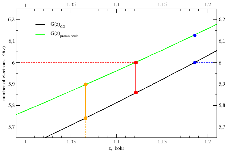
J. Am. Chem. Soc. 1970, 92, 6451-6454.] The black and green curves represent the electron-count function for the CO molecule and its promolecule, respectively. Vertical lines represent planes perpendicular to the interatomic axis. The coloured balls are the intersections of these planes with the electron-count functions.
In Figure 2, the red ball on the promolecule curve (green) is chosen in such a way its ordinate (i.e. the number of electrons on carbon) equals the number of protons in the carbon nucleus, ZC = 6. Its abscissa gives the position of the plane that separates the carbon atom from the oxygen atom, both in the promolecule and in the CO molecule, zboundary = 1.1212 bohr. Of course, the ordinate of the red ball on the molecule curve (black) gives the total number of electrons on the carbon in the CO molecule, G(zboundary)CO = 5.860 e. The difference of the ordinates of the two red balls gives the partial charge or net atomic charge of carbon in the CO molecule, q(C)Politzer = ZC − G(zboundary)CO = + 0.140 e. Politzer's rule is all here:
| q(atom)Politzer = G(zboundary)promol − G(zboundary)mol = Zatom − G(zboundary)mol | (13) |
where zboundary is required to satisfy the condition G(zboundary)promol = Zatom.
The result obtained for q(C)Politzer in CO is
consistent with (intermediate to) Mulliken and Lowdin atomic populations
calculated by GAMESS:
TOTAL MULLIKEN AND LOWDIN ATOMIC POPULATIONS
ATOM MULL.POP. CHARGE LOW.POP. CHARGE
1 C 5.715758 0.284242 5.916101 0.083899
2 O 8.284242 -0.284242 8.083899 -0.083899
Politzer recognized that his definition of atomic charge
“admittedly contains an element of arbitrariness in that the atomic regions could be defined in terms of other criteria than the requirement that the atoms have zero charges in the limit of no interaction.”[1Politzer, Peter; Harris, Roger R.
J. Am. Chem. Soc. 1970, 92, 6451-6454.]
Thus, if we select an arbitrary plane orthogonal to the internuclear axis and let it move like a cursor along that axis (cf the vertical lines in Figure 2), we obtain, for each z-value, the ordinates of the intersection points with the electron-count function of both the molecule and the promolecule. However, for an arbitrary value of the z coordinate, the last equality in eq (13) is not valid anymore. Instead, we obtain two separate equations that correspond to two different models:
| qVDD = −[ G(zboundary)mol − G(zboundary)promol ] = − [ zboundary ∫ −∞ g(z)mol dz − zboundary ∫ −∞ g(z)promol dz ] = − zboundary ∫ −∞ g(z)DD dz | (14) |
| qVP = Zatom − G(zboundary)mol = Zatom − zboundary ∫ −∞ g(z)mol dz | (15) |
Eq (14) defines the partial atomic charge due to the deformation density, g(z)DD = g(z)mol − g(z)promol, that is the density change when going from the superposition of atomic densities to the final molecular density. Eq (15) is the usual definition of partial atomic charge, i.e. the difference between the nuclear charge of the atom and the number of electrons assigned to it.
Having made zboundary free from fulfilling the condition
G(zboundary)promol =
Zatom, we are left with the problem to choose a reasonable
value for zboundary. To this aim and in view of future
generalizations, it is worth noting that Politzer's method, which uses planes
perpendicular to the internuclear axis to identify the boundaries of the atomic
regions, is an example of electron density partitioning into two (unbounded)
Voronoi polyedra (VP),[17Voronoi,
G. F.
Journal für die reine und angewandte Mathematik
1908, 134, 198-287.]
also known as Dirichlet[18Dirichlet,
G. L.
Journal für die reine und angewandte Mathematik
1850, 40, 209-227.] regions,
Wigner-Seitz[19Wigner, E. P.; Seitz, F.
Phys. Rev. 1933, 43, 804.] cells, or
domains.[20Frank, F. C.; Kasper, J. S.
Acta Crystallogr. 1958, 11, 184-190.]
For this reason, the net atomic charge in eqs (14) and (15) has been labeled
VDD and VP, respectively.
It should be noted that Voronoi deformation density (VDD) charges were
explicitly introduced by Fonseca Guerra and coworkers in 1996, [21(a) Bickelhaupt, F. M.; van Eikema Hommes, N. J. R.;
Fonseca Guerra, C.; Baerends, E. J.
Organometallics 1996,
15, 2923-2931.
(b) Fonseca Guerra, C.; Handgraaf, J.-W.;
Baerends, E. J.; Bickelhaupt, F. M.
J. Comput. Chem. 2004,
25, 189-210.
(c)Stasyuk, O. A.; Szatylowicz, H.; Krygowskib,
T. M.; Fonseca Guerra, C.
Phys. Chem. Chem. Phys. 2016,
18, 11624-11633.] using planes perpendicularly
bisecting internuclear axes.
Instead, Politzer's method not only underlies Voronoi partitioning (albeit
limited to linear molecules) but also anticipates an important extension in
which the position of the orthogonal boundary plane is no longer constrained
at the midpoint of the internuclear axis.[22Richards, F. M.
J. Mol. Biol. 1974,
82, 1-14.,
23Rousseau, B.; Peeters, A.; Van Alsenoy, C.
Journal of Molecular Structure (Theochem) 2001, 538,
235-238.,
26Alam, A.; Khan, S. N.; Wilson, B. G.;
Johnson, D. D.
Physical Review B 2011, 84,
045105.]
Indeed, in most materials, the midpoint criterion is a poor subdivision of
space, making VP corresponding to the smaller atoms too large, and to the
larger atoms too small.
Given these deficiencies, various proposals have been made to place the
dividing plane subject to atomic size.
In 1974 Richards[22Richards, F. M.
J. Mol. Biol. 1974, 82, 1-14.]
suggested using the ratio of the distance between atoms and dividing plane
to be equal to the ratio of the corresponding atomic radii,
| zboundary,A = RAB Rcov,A Rcov,B | (16) |
but this does not reflect bonding, as zboundary,A +
zboundary,B ≠ RAB, and the
space-filling property is not fulfilled. In 2001 Van Alsenoy and coworkers
removed this drawback by moving the perpendicular bisecting plane away from the
bond midpoint by a distance related to the relative sizes of the atoms:[23Rousseau, B.; Peeters, A.; Van Alsenoy, C.
Journal of Molecular Structure (Theochem) 2001, 538,
235-238.]
| zboundary,A = RAB Rvdw,A Rvdw,A + Rvdw,B | (17) |
where Rvdw,A, Rvdw,B and
RAB are the van der Waals radii of the atoms A and
B and the internuclear separation, respectively.
Since 1979 an alternative tessellation for packings of unequal spheres was
proposed, in order to be able to construct high density packings.[24Fisher, W.; Koch, E.
Z. Kristallogr. 1979, 150, 245-260.,
25Gellatly, B. J.; Finney, J. L.
J. Non-Cryst. Solids 1982, 50, 313-329.]
It is based on the Radical Plane Construction (RPC),[26Alam, A.; Khan, S. N.; Wilson, B. G.; Johnson, D. D.
Physical Review B 2011, 84, 045105.] which
leads to the following expression:[N3Radical
Plane Construction (RPC)]
| zboundary,A = RAB2 + rA2 − rB2 2 RAB | (18) |
where rA, rB and RAB are the radii of the spherical atoms A and B and the internuclear separation, respectively. If atoms A and B have the same size (rA = rB), the boundary plane is a perpendicular bisector of the internuclear axis (zboundary,A = ½RAB). Otherwise, the boundary plane is moved from the internuclear midpoint towards atom A or towards atom B depending of the sign of (rA − rB). If rA and rB are the atomic radii scaled in such a way their sum equals the bond length (rA + rB = RAB), as in eq (17), the atomic spheres centered at A and B are tangent at the point where the boundary plane intersects the internuclear axis perpendicularly (zboundary,A = RA).
Table 1 shows that an appropriate choice of the value of the atomic radii can be critical in finding a correct value of the atomic charge. This is all the more true if we think that small variations in the length of the radii determine small but significant variations in the value of the atomic charge and even a change in its sign.
| zboundary, bohr | rC⁄rO | G(zboundary)promol, e | G(zboundary)mol, e | qVDD, e | qVP, e |
|---|---|---|---|---|---|
| (a) rC = rO = ½rCO; (b) value such that Gpromol = 6 (Politzer's rule); (c) Bragg-Slater radii: rC = 0.70 Å and rO = 0.60 Å ["Atomic Radii in Crystals": Slater, J. C. J. Chem. Phys. 1964, 41, 3199-3204.] and eq. (17); (d) same parameters as (c), but with eq (18); (e) covalent radii from analysis of the Cambridge Structural Database: rC = 0.76 Å and rO = 0.66 Å ["Covalent radii revisited": Cordero, B.; Gómez, V.; Platero-Prats, A. E.; Revés, M.; Echeverría, J.; Cremades, E.; Barragán, F.; Alvarez, S. Dalton Trans. 2008, 2832-2838.] and eq. (17); (f) same parameters as (e), but with eq (18); (g) value such that Gmol = 6; (h) Clementi's covalent radii from SCF functions: rC = 0.67 Å and rO = 0.48 Å ["Atomic Screening Constants from SCF Functions. II. Atoms with 37 to 86 Electrons": Clementi, E.; Raimondi, D. L.; Reinhardt, W. P. J. Chem. Phys. 1967, 47, 1300-1307.] and eq. (17); (i) same parameters as (h), but with eq (18); (j) Gill-Johnson-Pople covalent radii: rC = 1.2308 bohr (0.651 Å) and rO = 0.8791 bohr (0.465 Å) ["A standard grid for density functional calculations": Gill, P. M. W.; Johnson, B. G.; Pople, J. A. Chem. Phys. Lett. 1993, 209, 506-512.] and eq. (17); (k) same parameters as (j), but with eq (18). | |||||
| 1.0661(a) | 1 | 5.895 | 5.740 | 0.155 | 0.260 |
| 1.1212(b) | − | 6.000 | 5.857 | 0.143 | 0.143 |
| 1.1481(c) | 1.167 | 6.053 | 5.915 | 0.137 | 0.085 |
| 1.1750(d) | 1.167 | 6.106 | 5.975 | 0.131 | 0.025 |
| 1.1412(e) | 1.152 | 6.039 | 5.900 | 0.139 | 0.100 |
| 1.1850(f) | 1.152 | 6.126 | 5.998 | 0.129 | 0.002 |
| 1.1863(g) | − | 6.129 | 6.000 | 0.129 | 0.000 |
| 1.2422(h) | 1.396 | 6.245 | 6.129 | 0.116 | −0.129 |
| 1.2491(i) | 1.396 | 6.259 | 6.145 | 0.114 | −0.145 |
| 1.2438(j) | 1.400 | 6.248 | 6.133 | 0.115 | −0.133 |
| 1.2401(k) | 1.400 | 6.240 | 6.124 | 0.116 | −0.124 |

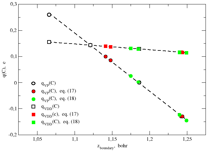
It appears from Table 1 and Figure 4 that
qVDD(C) decreases by only 0.041 e in the range of
z-values considered (about 0.2 bohr), whereas
qVP(C) decreases by 0.405 e and changes its sign.
There is no reason to wonder about this result, because the two quantities are
non consistent with each other. Really, qVP measures the gain or loss of electrons of an atom in a molecule with respect to the isolated
atom. On the other hand qVDD measures the difference of the
gross atomic charge of an atom in a molecule and the gross atomic charge of
the same atom in the promolecule.
The promolecule density does not differ very much from the
final molecular density,[27Spackman, M. A.;
Maslen, E. N.
J . Phys. Chem. 1986, 90,
2020-2027., 28Maslen, E. N.;
Spackman, M. A.
Aust. J. Phys. 1985, 38,
273-87.] and the same can be said for many chemical properties
derived from them. This can lead to mistakenly interpreting, as binding
interactions in the molecule, properties which are already present in the
promolecule. [27Spackman, M. A.;
Maslen, E. N.
J . Phys. Chem. 1986, 90,
2020-2027.]
The deformation density quantitatively monitors how chemical
properties change on passing from the promolecule to the final molecule, but
says nothing about the actual amount of their values.
Anyway, the small rate of variation of deformation density charges with respect
to the position of the boundary plane justifies using bisecting planes as VP
faces.
On the other hand, calculation of net atomic charges generally requires that
the position of VP faces depends on the atom size.
Extension to non-linear molecules.
For molecules with a three-dimensional structure, the electron density is better expressed in terms of spherical coordinates.[L5PAMoC manual. “Methods of Numerical Integration: § 2 - Volume integral”.] The number of electrons (i.e. the total electronic charge) of the molecule still retains the form of eq (2),
| N = ∫ V ρ(r) d3r = +∞ ∫ 0 g(r) dr | (19) |
but now g(r) represents the radial probability density (or radial electron density distribution) of a spherical shell volume element of infinitesinal thickness and radius r:
| g(r) = r2 σ(r) | (20) |
where σ(r) is the spherically averaged probability density (or spherically averaged electron density distribution) of an infinitesinal volume element at point r:
| σ(r) = π ∫ 0 sinθ dθ 2π ∫ 0 ρ(r,θ,φ) dφ = ∫ Ω ρ(r,Ω) dΩ | (21) |
where the solid angle Ω is the two-dimensional angle in three-dimensional space that an object subtends at a point. It is equal to the area of the segment of a unit sphere, centered at the angle's vertex.
As in equation (1), the quantities in eqs (19-21) can be partitioned into atomic contributions. However Politzer's definition of AIM cannot be applied strictly or unambiguously to the atoms of a non-linear promolecule.
It might be tempting to integrate the electron density of the promolecule over a sphere centered on atom A and with a radius such that the value of the electron density in this sphere is equal to ZA. Unfortunately, as expected, such a sphere ends up incorporating almost the whole molecule (see figure on the left). This means that the model is unrealistic and therefore unacceptable.
.
Radical Plane Construction (RPC) uses the weighted metric ∥P − Qi∥2 − ri2, where ri is the radius of the i-th atom and ∥P − Qi∥2 is the Euclidean distance between point P and atom center Qi. The advantage of the RPC tessellations is that the resulting domains are guaranteed to be convex polyhedra [B.J. Gellatly and J.L. Finney, J. Non-Cryst. Solids 50, 313 (1981).] whose inscribed spheres match the input radii {ri}.
The proposed definition for region i is ∥P − Qi∥2 − ri2 < ∥P − Qj∥2 − rj2 ∀ j ≠ i.
This essellation is ideally suited for studying the void space in-between spheres, because of its following properties:
(1) The boundaries between regions are planar. The boundary between regions i and j is perpendicular to the line connecting Qi and Qj .
(2) For equal spheres this is the Voronoi tessellation.
(3) For overlapping spheres the boundary between regions coincides with the plane of intersection of the spheres.
(4) For nonoverlapping spheres the boundary between regions always lies between the spheres (which is not valid for the Voronoi tessellation applied to unequal spheres).
(5) The proof by Kerstein holds for arbitrary radii.
The latter point can be explained as follows. Consider a point P inside polyhedron i, but outside its associated sphere. I show that P lies in the void space. For the proposed tessellation P has the properties
∥P − Qi∥ − ri > 0.
∥P − Qi∥2 − ri2 < ∥P − Qj∥2 − rj2 ∀ j ≠ i.
From the first line it follows that ∥P − Qi∥2 − ri2 > 0. Using the second line I conclude that ∥P − Qj∥2 − rj2 > 0 and hence ∥P − Qj∥ > rj for all j. In other words, the point P lies outside all spheres and hence in the void space.
This tessellation also has a new property: polyhedron i need no longer contain the center of sphere i. In fact, a region can be entirely empty, which is not possible with the Voronoi tessellation. This does not pose a problem, however, because a region will be empty only if its associated sphere is located entirely within one or more other spheres: in those cases one could of course have “thrown away” that sphere in the first place. [Network Approach to Void Percolation in a Pack of Unequal Spheres S. C. van der Marck PHYSICAL REVIEW LETTERS 1996 77 1785 1788]
The boundary plane between two atoms A and B can be defined as the "radical plane of two spheres" with radius Ra and Rb,respectively. The radical plane of two spheres is that plane, the points of which have equal tangential distances to both spheres (see Fig. 2). The polyhedra constructed in this way are always convex and the space-filling property is maintained in addition.[W. Fisher and E. Koch, Z. Kristallogr. 150 (1979) 245-260.] Definition of radical plane : a plane that is the locus of points from which tangents drawn to two given spheres are equal È detto piano radicale il luogo geometrico dei punti che hanno la stessa potenza rispetto a due sfere; se le due sfere hanno punti in comune, il piano radicale è quello che contiene la circonferenza intersezione.
Although in general the choice of the midpoint of the internuclear axis
would be rather unrealistic,[1Politzer, Peter; Harris, Roger R.
J. Am. Chem.
Soc. 1970, 92, 6451-6454.] and indeed
in the case of CO the criterion proposed by Politzer and Harris finds a
boundary plane placed 0.0551 bohr beyond the bond midpoint
(½ rCO = 1.0661 bohr), and actually this is not
even enough, because it would be necessary to move the boundary plane at
z > bohr to find a partial negative charge on the carbon, as it was
observed experimentally.[17Muenter, J. S.
J. Mol. Spectr. 1975, 55, 490-491.]
On the other hand,
placing the boundary plane at z = ½ rCO.
References
- (a) “Properties of Atoms in Molecules. I. A Proposed
Definition of the Charge on an Atom in a Molecule”
Politzer, Peter; Harris, Roger R. J. Am. Chem. Soc. 1970, 92, 6451-6454.
(b) “Properties of Atoms in Molecules. The Position of the Center of electronic Charge of an Atom in a Molecule”
Politzer, P.; Stout, Jr., E. W. Chem. Phys. Lett. 1971, 8, 519-522.
(c) “Properties of Atoms in Molecules. III. Atomic Charges and Centers of Electronic Charge in some Heteronuclear Diatomic Molecules”
Politzer, P. Theor. Chim. Acta 1971, 23, 203-207. - “Chemically Meaningful Atomic Charges That Reproduce the
Electrostatic Potential in Periodic and Nonperiodic Materials”
Manz, T. A.; Sholl, D. S. J. Chem. Theory Comput. 2010, 6, 2455-2468. - “Modeling the Partial Atomic Charges in Inorganometallic
Molecules and Solids and Charge Redistribution in Lithium-Ion
Cathodes”
Wang, B.; Li, S. L.; Truhlar, D. G. J. Chem. Theory Comput. 2014, 10, 5640−5650. - “A Test of Various Partial Atomic Charge Models for
Computations on Diheteroaryl Ketones and Thioketones”
Matczak, P. Computation 2016, 4, 3. - “Classical Electrostatics for Biomolecular Simulations”
Cisneros, G. A.; Karttunen, M.; Ren, P.; Sagui, C. Chem. Rev. 2014, 114, 779-814. - “Electrostatic Interactions in Protein Structure, Folding,
Binding, and Condensation”
Zhou, H.-X.; Pang, X. Chem. Rev. 2018, 118, 1691-1741. - Stone, A. J. “The Theory of Intermolecular Forces”
Oxford University Press, Oxford, 2000, ISBN 0-19-855883-X. - “Atomic Charges Are Measurable Quantum Expectation Values:
A Rebuttal of Criticisms of QTAIM Charges”
Bader, R. F. W.; Matta, C. F. J. Phys. Chem. A 2004, 108, 8385-8394. - “Electronic Population Analysis on LCAOMO Molecular Wave
Functions. I”
Mulliken, R. S. J. Chem. Phys. 1955, 23, 1833-1840. - (a) “Electronic Structures of Polyatomic Molecules
and Valence”
Mulliken, R. S Phys. Rev. 1932, 40, 55-62.
(b) “Electronic Structures of Polyatomic Molecules and Valence. II. General Considerations”
Mulliken, R. S. Phys. Rev. 1932, 41, 49-71a - “Electronic Structures of Molecules. XI. Electroaffinity,
Molecular Orbitals and Dipole Moments”
Mulliken, R. S. J. Chem. Phys. 1935, 3, 573-585, Eqs. (38), (39), (42). - “More reliable partial atomic charges when using diffuse
basis sets.”
Thompson, J.D.; Xidos, J.D.; Sonbuchner, T.M.; Cramer, C.J.; Truhlar, D.G. PhysChemComm 2002, 5, 117–134. - “Comparison of Two Atomic Charge Definitions, as Applied
to the Hydrogen Fluoride Molecule”
Politzer, P.; Mulliken, R. S. J. Chem. Phys. 1971, 55, 5135-5136. - “A Configuration Interaction Study of the Four Lowest
1Σ+ States of the LiH Molecule”
Brown, Richard E.; Shull, Harrison Int. J. Quantum Chem. 1968, 2, 663-685. - (a) “Observed adiabatic corrections to the
Born-Oppenheimer approximation for diatomic molecules with ten
valence electrons”
Tiemann, E.; Arnst, H.; Stieda, W. U.; Törring, T.; Hoeft, J. Chem. Phys. 1982 67, 133-138.
(b) “Electronic Structure of CO − An Exercise in Modern Chemical Bonding Theory”
Frenking,G.; Loschen, C.; Krapp, A.; Fau, S.; Strauss, S. H. J. Comput. Chem. 2007, 28, 117-126.
(c) “Equilibrium CO bond lengths”
Demaison, J.; Császár, A. G. J. Mol. Struct. 2012, 1023, 7-14. - “Electrostatic binding in the first-row AH and A2
diatomic molecules”
Hirshfeld, F. L.; Rzotkiewicz, S. Mol. Phys. 1974, 27, 1319-1343. - “Nouvelles applications des paramètres continus
à la théorie des formes quadratiques. Deuxième
mémoire. Recherches sur les parallélloèdres
primitifs.”
Voronoi, G. F. Journal für die reine und angewandte Mathematik 1908, 134, 198-287. - “Über die Reduction der positiven quadratischen Formen
mit drei unbestimmten ganzen Zahlen.”
Dirichlet, G. L. Journal für die reine und angewandte Mathematik 1850, 40, 209-227. - “On the Constitution of Metallic Sodium.”
Wigner, E. P.; Seitz, F. Phys. Rev. 1933, 43, 804. - “Complex alloy structures regarded as sphere packings. I.
Definitions and basic principles.”
Frank, F. C.; Kasper, J. S. Acta Crystallogr. 1958, 11, 184-190. - (a) “The Carbon-Lithium Electron Pair Bond in
(CH3Li)n (n = 1, 2, 4)”
Bickelhaupt, F. M.; van Eikema Hommes, N. J. R.; Fonseca Guerra, C.; Baerends, E. J. Organometallics 1996, 15, 2923-2931.
(b) “Voronoi Deformation Density (VDD) Charges: Assessment of the Mulliken, Bader, Hirshfeld, Weinhold, and VDD Methods for Charge Analysis”
Fonseca Guerra, C.; Handgraaf, J.-W.; Baerends, E. J.; Bickelhaupt, F. M. J. Comput. Chem. 2004, 25, 189-210.
(c) “How amino and nitro substituents direct electrophilic aromatic substitution in benzene: an explanation with Kohn-Sham molecular orbital theory and Voronoi deformation density analysis”
Stasyuk, O. A.; Szatylowicz, H.; Krygowskib, T. M.; Fonseca Guerra, C. Phys. Chem. Chem. Phys. 2016, 18, 11624-11633. - “The Interpretation of Protein Structures: Total Volume,
Group Volume Distributions and Packing Density”
Richards, F. M. J. Mol. Biol. 1974, 82, 1-14. - “Atomic charges from modified Voronoi polyhedra”
Rousseau, B.; Peeters, A.; Van Alsenoy, C. Journal of Molecular Structure (Theochem) 2001, 538, 235-238. - “Geometrical packing analysis of molecular
compounds”
Fisher, W.; Koch, E. Z. Kristallogr. 1979, 150, 245-260. - “Characterisation of models of multicomponent amorphous
metals: the radical alternative to the Voronoi polyhedron”
Gellatly, B. J.; Finney, J. L. J. Non-Cryst. Solids 1982, 50, 313-329. - “Efficient Isoparametric Integration over Arbitrary,
Space-Filling Voronoi Polyhedra for Electronic-Structure
Calculations”
Alam, A.; Khan, S. N.; Wilson, B. G.; Johnson, D. D. Physical Review B 2011, 84, 045105. - “Chemical Properties from the Promolecule”
Spackman, M. A.; Maslen, E. N. J . Phys. Chem. 1986, 90, 2020-2027. - “Atomic Charges and Electron Density Partitioning”
Maslen, E. N.; Spackman, M. A. Aust. J. Phys. 1985, 38, 273-87. - “Electric Dipole Moment of Carbon Monoxide”
Muenter, J. S. J. Mol. Spectr. 1975, 55, 490-491.
Notes
- Population Analysis of Wave Functions. In the
Born-Oppenheimer approximation, the solution of the Schrödinger
equation for a molecular entity, is the electronic wavefunction
Ψ(r1,r2,…,rN,ω1,ω2,…ωN),
which is a function of the vectorial positions ri
and spins ωi of the N electrons of the
molecular entity. The wave function must be antisymmetric under exchange
of any two of the electrons in order to satisfy the Pauli exclusion
principle. This is accomplished by defining the electronic wave function
as a Slater determinant of properly chosen orthogonal molecular orbital (MO)
wave functions of the individual electrons,
Φi(rj,ωj) ∀ i,j = 1,2,…,N :
where in the final expression a compact notation is introduced that only exhibits MO wave functions. The Slater determinant is a linear combination of Hartree products of N MO's (orbital approximation), which together with approximating the electronic Hamiltonian with the sum of N effective one-electron Hamiltonian operators (mean field approximation) breaks down the electronic Schrödinger equation, partial differential equation of a function of N variables, into a system of N independent partial differential equations of functions of one variable only (one-electron Schrödinger equations). To find the MO wave functions, { Φi }, and the associated MO energies, { εi }, each MO is approximated with a linear combination of atomic orbitals (LCAO):Ψ(r1,r2,…,rN,ω1,ω2,…ωN) = (N!)−½
≡ |Φ1,Φ2,…,ΦN⟩,Φ1(r1,ω1) Φ2(r1,ω1) … ΦN(r1,ω1) Φ1(r2,ω2) Φ2(r2,ω2) … ΦN(r2,ω2) ⋮ ⋮ ⋱ ⋮ Φ1(rN,ωN) Φ2(rN,ωN) … ΦN(rN,ωN)
The oldest and most influential procedure of this kind has been proposed by Mulliken:[9Mulliken, R. S.Φ = ∑ i ci χi.
J. Chem. Phys. 1955, 23, 1833-1840.]
where Sij = <χi|χj> and Dij are the overlap integrals and the one-electron density matrix elements, respectively, with respect to the basis atomic orbitals χi and χj, the χj∈A ones being somewhat artificially assigned to atom A. The resulting nonuniqueness and artifacts are well-known.30qA(MPA) = ZA − ∑ i, j∈A DijSij These drawbacks partially arise from the fact that the Mulliken population analysis utilizes a nonorthogonal basis set. This problem is overcome by the natural population analysis (NPA)[Foster, J. P.; Weinhold, F. “Natural hybrid orbitals.” J. Am. Chem. Soc. 1980, 102, 7211−7218.][Reed, A.E.; Weinstock, R.B.; Weinhold, F. “Natural population analysis.” J. Chem. Phys. 1985, 83, 735–746.][Reed, A.E.; Curtiss, L.A.; Weinhold, F. “Intermolecular interactions from a natural bond orbital, donor-acceptor viewpoint.” Chem. Rev. 1988, 88, 899–926.] in which orthonormal natural atomic functions are constructed. The distributed multipole analysis of Gaussian wave functions (GDMA) [Stone, A.J. “Distributed multipole analysis: Stability for large basis sets.” J. Chem. Theory Comput. 2005, 1, 1128–1132.] is also ranked among the models of the first group.
Mulliken 16 and minimum basis set (MBS) Mulliken 22[Montgomery, J. A.; Frisch, M. J.; Ochterski, J. W.; Petersson, G. A. “A complete basis set model chemistry. VII. Use of the minimum population localization method.” J. Chem. Phys. 2000, 112, 6532−6542.] charges are based on partitioning of the overlap matrix of atomic orbitals. Since Mulliken charges are very sensitive to the basis sets, the MBS Mulliken charge algorithm was developed to improve the partition by mapping the charge density to the minimum basis set, which gives a more balanced description among atoms and ameliorates some instability problems of Mulliken charges. 22
Natural population analysis (NPA) charges 19 use natural bond orbitals with maximum electron density and natural atomic orbitals to localize the electrons to atoms. This reduces the basis-set dependence.
LoProp charges 23[Gagliardi, L.; Lindh, R.; Karlström, G. “Local properties of quantum chemical systems: The LoProp approach.” J. Chem. Phys. 2004, 121, 4494−4500.] are derived by the orthogonalization of the original basis set to get a set of localized orthonormal basis set. (This may be an improvement over the Löwdin scheme, 38[L&ounl;wdin, P.-O. “On the non-orthogonality problem connected with the use of atomic wave functions in the theory of molecules and crystals.” J. Chem. Phys. 1950, 18, 365−375.],39[Li, J.; Zhu, T.; Cramer, C. J.; Truhlar, D. G. “New Class IV Charge Model for Extracting Accurate Partial Charges from Wave Functions.” J. Phys. Chem. A 1998, 102, 1820−1831.] in that it involves three or four separate and specialized Löwdin orthonormalizations, and it may be an improvement over natural atomic orbital analysis, in that it depends only on geometry, not on electron configuration). - Electron density. Quantum mechanics provides a recipe for calculating the probability ρ(x,y,z) dx dy dz to find an electron in an element of volume dV = dx dy dz at a particular point in space with coordinates x, y, z, and this quantity is expressed in terms of a function ρ(x,y,z) called "probability density" or "electronic density". Because of the Heisemberg uncertainty principle, we can not say exactly where the electron is, but only calculate the probability that it is in a volume element dV around a particular point in space. This does not imply that the electron is "diluted" throughout the region of space in which the electronic density is non-zero: in a certain volume dV there may be a very small probability of finding the electron; but if you find it there, you find it entirely. However, in many cases (for example, dispersion of X-rays, forces on atoms), a system consisting of a large number of electrons behaves exactly as if the electrons were distributed over a region of space, so that each point in space is characterized by a certain fraction of charge or partial charge, which can be called "charge density" or "electronic density" and is identical to the probability density. In fact, for large numbers, the frequency tends to probability. Therefore, a map showing how the probability density varies from point to point in a molecule, ie a map of the total electron density, ie of the cumulative distribution of the charge of all the electrons of the molecule, is a model of the electronic structure of the molecule.
- Voronoi Polyhedra.
Voronoi polyhedra are intersections of half-spaces; they are convex but
not necessarily bounded. A half-space is either of the two parts into
which a plane divides the three-dimensional Euclidean space. That is, the
points that are not incident to the plane are partitioned into two convex
sets (i.e., half-spaces), such that any subspace connecting a point in one
set to a point in the other must intersect the plane.
Voronoi polyhedra can be constructed in the following manner. Consider a set of points P1, P2, …, Pn in the three-dimensional Euclidean space ℝ. Consider the line interconnecting the point Pi and one of its neighbors Pj. Construct a plane hij perpendicular to this line at its midpoint zij. Repeating this process for all points Pj yields a set of planes that define a polyhedron around point Pi. The set of Voronoi polyhedra corresponding to a given configuration of centers is called the Voronoi diagram.
So, the Voronoi polyhedron Vi around a given center Pi, is the set of points in ℝ closer to Pi than to any Pj: more formally,
where d denotes distance. We call Hij the half-space generated by hij that consists of the subset of ℝ on the same side of hij as Pi; that is,Vi = {x ∈ ℝ : d(x, Pi) ≤ d(x, Pj), j = 1, 2 , …, n}, (N2.1)
Vi is bounded by faces, with each face fij belonging to a distinct plane hij. Each face is characterized by listing its vertices and edges in cyclic order.Vi = ⋂ j Hij. (N2.2)
[Source of this note is paper “Construction of Voronoi Polyhedra” by Witold Brostow and Jean-Pierre Dussault on the Journal of Computational Physics, 1978, 29, 81-92.] - Radical Plane Construction (RPC).
This note is intended to derive the Cartesian coordinates of the
intersection point of the radical plane of two spheres, centered on points
A and B, with the line passing through
A and B. It is also a review of some
fundamental notions of analytic geometry.
Definition of sphere in three-dimensional space. Given a point C = (xC, yC, zC) and a scalar rC > 0, we define sphere S(C,rC) of center C and radius rC the locus of points P = (x, y, z) such that their distance from C is equal to rC, i.e. |P − C| = rC, or also |P − C|2 = rC2, from which we obtain the Cartesian equation of the sphere in three-dimensional space
that is, doing the calculations(x − xC)2 + (y − yC)2 + (z − zC)2 = rC2 (N3.1)
The latter equation can also be written in the formx2 + y2 + z2 − 2xCx − 2yCy − 2zCz + xC2 + yC2 + zC2 − rC2 = 0 (N3.2)
where we have setx2 + y2 + z2 + αx + βy + γz + δ = 0 (N3.3)
More formally, the setα = − 2xC, β = − 2yC, γ = − 2zC, δ = xC2 + yC2 + zC2 − rC2 (N3.4)
is a sphere S = S(C,rC) of centerS = { (x, y, z) | x2 + y2 + z2 + αx + βy + γz + δ = 0 } (N3.5)
and radiusC = ( − α 2, − β 2, − γ 2 ) (N3.6)
provided thatrC = √ α2 + β2 + γ2 − 4δ 2 (N3.7) α2 + β2 + γ2 − 4δ > 0 (N3.8) Intersection of two spheres. Let S(A,rA) and S(B,rB) two non-concentric spheres (A ≠ B). The coordinates of the points that satisfy the two equations of S(A,rA) and S(B,rB)
also satisfy the equation obtained by subtracting the two equations from each other.x2 + y2 + z2 + αAx + βAy + γAz + δA = 0 (N3.9) x2 + y2 + z2 + αBx + βBy + γBz + δB = 0
This equation represents a plane, called the radical plane of the pair of spheres SA and SB, which is perpendicular to(αA − αB)x + (βA − βB)y + (γA − γB)z + (δA − δB) = 0 (N3.10) (A − B) = (αA − αB)i + (βA − βB)j + (γA − γB)k (N3.11) Intersection of a plane with a straight line passing through two known points. For simplicity, suppose that points A and B lie both on the z-axis, e.g. A = (0, 0, zA) and B = (0, 0, zB), and let C = (0, 0, zboundary) be the point of intersection of the radical plane with the straight line passing through A and B. Replacing the coordinates of C in the equation of the radical plane, and solving with respect to zboundary, yields
It is worth noting that if the two non-concentric spheres S(A,rA) and S(B,rB) have the same radius (rA = rB), the point of intersection is the middle point of the segment AB. If the sum of the radii is less than the distance of the centers (rA + rB < zB − zA), the two spheres do not intersect. Vice versa, if the sum of the radii is greater than the distance of the centers (rA + rB > zB − zA), the intersection of the two spheres is a circumference contained in the radical plane. Finally, if the sum of the radii is equal to the distance of the centers (rA + rB = zB − zA), the two spheres are tangent to a point which belongs to the radical plane. Equation (N3.12) can be applied directly to the specific case of carbon monoxide.zboundary = δB − δA γA − γB = zB2 − zA2 + rA2 − rB2 2(zB − zA) = zA + zB 2 + rA2 − rB2 2(zB − zA) (N3.12) In order to find the coordinates of the intersection point in the general case, let's start from the vector equation of the line that joins the two centers
which is equivalent to three scalar equations for the three components of vectors P, A e B (this set of equations is called the parametric form of the equation of a line). Solving each of the equations in the parametric form of the line for t, and setting all of them equal to each other since t will be the same number in each, yields the symmetric equations of the lineP = A + (B − A) t (N3.13)
Choosing two of the three possible symmetric equations and combining them together to the equation of the radical plane, gives the following matrix equationx − xA xB − xA = y − yA yB − yA = z − zA zB − zA (N3.14)
from which we getΔγ 0 − Δα 0 Δγ − Δβ Δα Δβ Δγ
=xboundary yboundary zboundary xAΔγ − zAΔα yAΔγ − zAΔβ − Δδ (N3.15)
so that the coordinates of the intersection point turn out to have the following expression
= [ Δγ (Δα2 + Δβ2 + Δγ2) ]−1xboundary yboundary zboundary Δβ2 + Δγ2 − Δα Δβ Δα Δγ − Δα Δβ Δα2 + Δγ2 Δβ Δγ − Δα Δγ − Δβ Δγ Δγ2 xAΔγ − zAΔα yAΔγ − zAΔβ − Δδ (N3.16)
where the following equality and definitions have been usedcboundary = cA − (cB − cA) A ⋅ Δ + Δδ 2 RBA2 = cA + (cB − cA) RBA2 + rA2 − rB2 2 RBA2, ∀ c = x, y, z (N3.17)
It can be readily verified that equation (N3.12) is a special case of eq (N3.17). The procedure followed to obtain this result has proven to be rather cumbersome. The same result can be achieved in a similar and faster way. To this aim, we rewrite eqs (N3.10) and (N3.13) as followsΔα = αA − αB = 2 (xB − xA), Δβ = βA − βB = 2 (yB − yA), Δγ = γA − γB = 2 (zB − zA),
Δδ = δA − δB = − (B − A) ⋅ (A + B) − (rA2 − rB2) = − A ⋅ Δ − (B − A)2 − (rA2 − rB2) = − A ⋅ Δ − RBA2 − (rA2 − rB2),
Δ = ( Δα, Δβ, Δγ ) = 2 (B − A),
Δ2 = Δα2 + Δβ2 + Δγ2 = 4 [ (xB − xA)2 + (yB − yA)2 + (zB − zA)2 ] ≡ 4 RBA2,(N3.18)
andΔ ⋅ P = − Δδ (N3.19)
Plugging in gives the equationP = A + Δ 2t (N3.20)
from which the parameter t is derivedΔ ⋅ A + Δ2 2t = − Δδ (N3.21)
Plugging eq (N3.22) in eq (N3.13) gives the equationt = − 2 Δ ⋅ A + Δδ Δ2 = RBA2 + rA2 − rB2 2 RBA2 (N3.22)
which is equivalent to eq (N3.17). From eq (N3.33), the distance of point P from the origin A is readily obtainedP = A + (B − A) RBA2 + rA2 − rB2 2 RBA2 (N3.33)
Eq (N3.12) is a special case of eq (N.34).D = | P − A | = RBA2 + rA2 − rB2 2 RBA = RBA 2 + rA2 − rB2 2 RBA (N3.34) Even more simply and quickly, it would have been enough to observe[L4Weisstein, Eric W. “Plane.”
From MathWorld − A Wolfram Web Resource.] that a plane specified by eq (N3.10) has x-, y-, and z-intercepts at
and lies at a distancex = − Δδ Δα, y = − Δδ Δβ, z = − Δδ Δγ, (N3.35)
from the origin (0,0,0). If we assume that point A is located at the origin, e.g. A = (0,0,0), then eq (N3.36) takes the expression of eq (N3.34).D = Δδ √ Δα2 + Δβ2 + Δγ2 (N3.36) Otherwise it would have been enough to remember[L4Weisstein, Eric W. “Plane.”
From MathWorld − A Wolfram Web Resource.] that the (signed) distance from a point A = (−αA/2, −βA/2, −γA/2) to the plane (N3.10) is
which gives the same result as eq (N3.34). The distance is positive if A is on the same side of the plane as the normal vector Δ and negative if it is on the opposite side.D = Δ ⋅ A + Δδ |Δ| - Promolecule. The promolecule is an ideal reference system made up by non-interacting atoms placed at the same positions they occupy in the molecule. Then the promolecule density is a superposition of the free-atom electron densities (usually spherically averaged) centred at the positions of the atoms in the molecule.
Links
-
 Dr. Peter Politzer's page (http://www.clevetheocomp.org/peter.html)
and publications (https://www.researchgate.net/scientific-contributions/38975283_Peter_Politzer/publications).
Accessed 12 Jan 2018.
- PAMoC manual. “Charge Distributions: § 4.6 - Transformation of the Random Vector Variable”, equation (4.6.8). Online resource: https://www.pamoc.it/tpc_chg_dstr.html#TRV.
- “GAMESS: General Atomic and Molecular Electronic Structure
System”. Online resource: http://www.msg.ameslab.gov/gamess/.
Accessed 1 Dec 2017.
- “Plane ”, by Weisstein, Eric W.
From MathWorld − A Wolfram Web Resource: http://mathworld.wolfram.com/Plane.html. Accessed 3 Mar 2018. - PAMoC manual. “Methods of Numerical Integration: § 2 - Volume integral”. Online resource: https://www.pamoc.it/tpc_num_int.html#VOL.